Answer Extractions: Engineering a Locator

When decider models, or “system one” models, arrived in everyone’s feeds, thanks largely to Jev and TypeSafe, what excited me wasn’t that AI engineers had one new model to look at. It was the implication: that we’d shortly see more small models doing other tasks faster and more cheaply than a general LLM can. Not one model that does everything, but a toolkit of small, efficient models that each do one common language task well, which an engineer orchestrates.

When we launched Strands Decider, the best part was that all of it was open, training code, data, and the research record, so anyone could rebuild it or push it somewhere new. The community promptly did: image deciders, audio deciders, bigger deciders. That’s the point of shipping the method rather than the weights.

But I wanted a different task entirely, using the same pattern. So for the last while I’ve been building what I’m calling a locator.

What is a locator?

It takes a document and a question. It returns the character offsets of the span of the document that answers the question, [887, 984], or a flag saying the answer isn’t in there.

That’s it. No generated text. The answer is a slice of the document by construction.

The appeal is that it cannot hallucinate, because it never produces a token. It can absolutely be wrong, it can point at the wrong clause, and it does, but it can only ever hand you back something that was already on the page, or an admission that nothing on the page fits.

I should be careful with the credit here. That faithfulness is a property of extractive question answering in general, not of my model in particular. The RoBERTa baseline (I’ll get to in a minute) also scores a perfect 1.0000 on “is the returned span really a substring”, for exactly the same reason. What I have to argue is that mine is more accurate, generalises better, and is better at refusing. Not that it’s uniquely honest.

How does it work?

Take a pretrained decoder, a 2B Qwen3.5, and never construct its language-modelling head at all. Bolt on a 2.63M-parameter span pointer in its place. The torso is frozen; only rank-16 LoRA adapters and the head train.

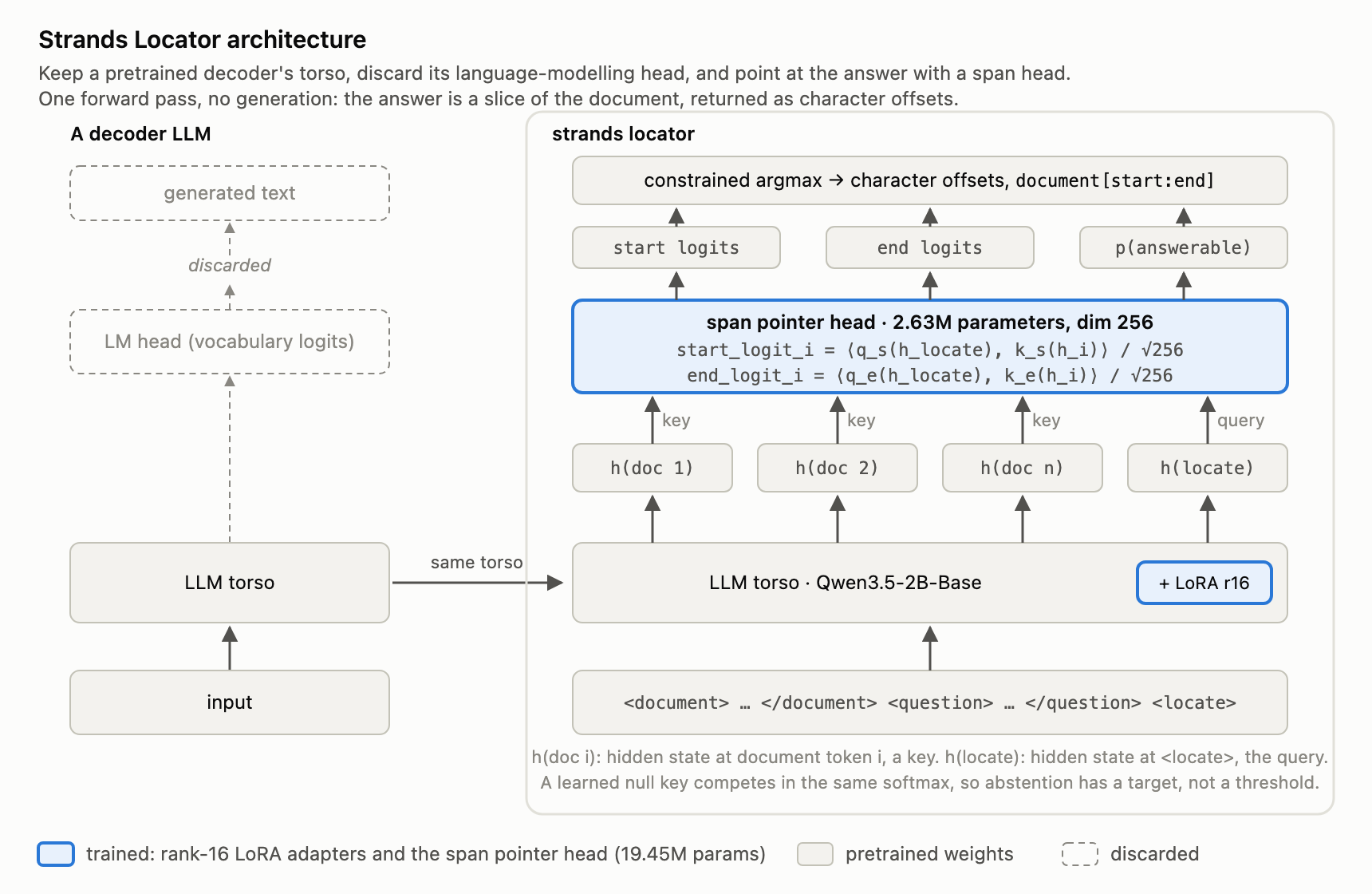The language modelling head is never constructed. A 2.63M-parameter span pointer takes its place, and the readout is character offsets rather than text.

The document goes in first, then the question, then a <locate> marker. The hidden state at that marker has read both, so it works as a query vector: score every document position for being a start, score every position for being an end, take the best start ≤ end pair under a length cap as a single masked argmax. One forward pass, no decoding loop. A learned null key competes in the same softmax, which is what gives “nothing here answers this” a well-defined target rather than a threshold bolted on afterwards.

Why a pointer and not two linear classifiers over the document? Because with the document placed first, a document token’s hidden state hasn’t attended to the question yet. A linear head would be scoring “is this token answer-shaped in general”, not “does this token answer this question.” That distinction turns out to be the whole ballgame, and I’ll come back to it, because I trained the weak version on purpose.

Does the BERT argument actually hold?

Here’s the contention I started with. Encoder models, BERT, RoBERTa, are tiny and fast and genuinely good at a range of extraction tasks. My claim was that they fall down once the question gets linguistically nuanced: where is this customer hinting they might leave?, which sentence quietly expands the scope? Questions whose words don’t appear anywhere near the answer. This is the same argument people have about whether deciders need to exist at all given that BERT is right there.

I’ve now run that comparison properly, on real documents, and I was partly wrong, in a way some are trying to convince me I find more interesting than being right. :)

The dataset is 46,402 training rows built on real, human-written documents, UK Hansard, Stack Exchange, SEC EDGAR, Wikipedia Talk, chosen because the document existed before the question did, written by a person for their own purposes. No generator can shape the text to suit the query. Against that, I fine-tuned deepset/roberta-base-squad2 on the identical rows, three seeds, all 124M of its parameters trainable against the locator’s 19.45M, and scored both sides through one harness. I should be clear that the locator is the bigger model here in every sense that matters for cost: 2B resident against 125M, and eight times the trainable parameters. It ought to win.

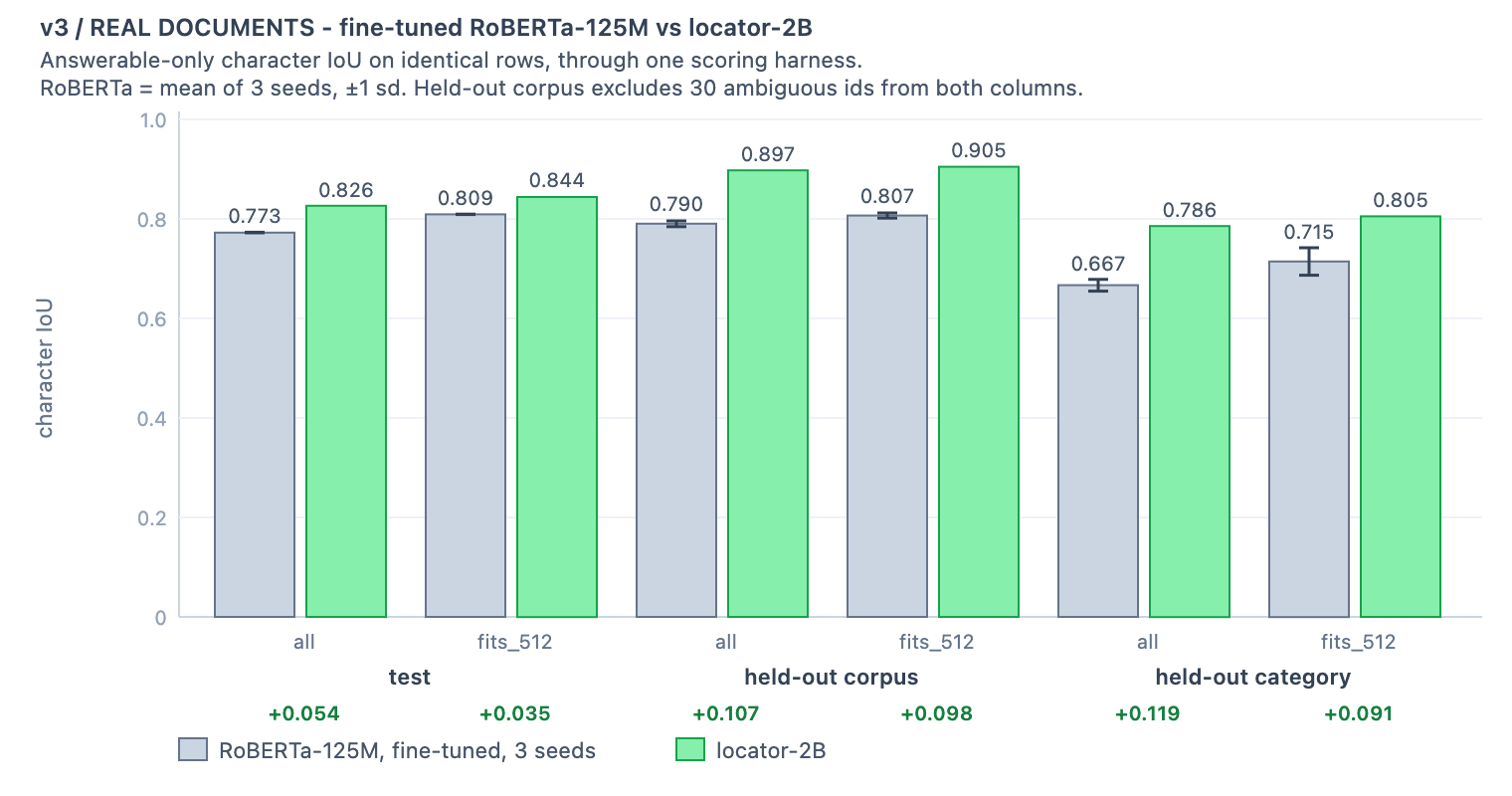
Real documents. Both columns through one scoring harness, so the only difference is the model.

The locator wins everywhere I measured. But on the main test set, on the subset of documents short enough that RoBERTa sees every character, it wins by +0.035 character IoU. That is much, much closer than I expected.

Why did I carry on when I got those numbers? Well, on the previous, synthetic version of this dataset, that same measurement, same two architectures, same subset definition, came out at +0.182. So I got a bit excited.

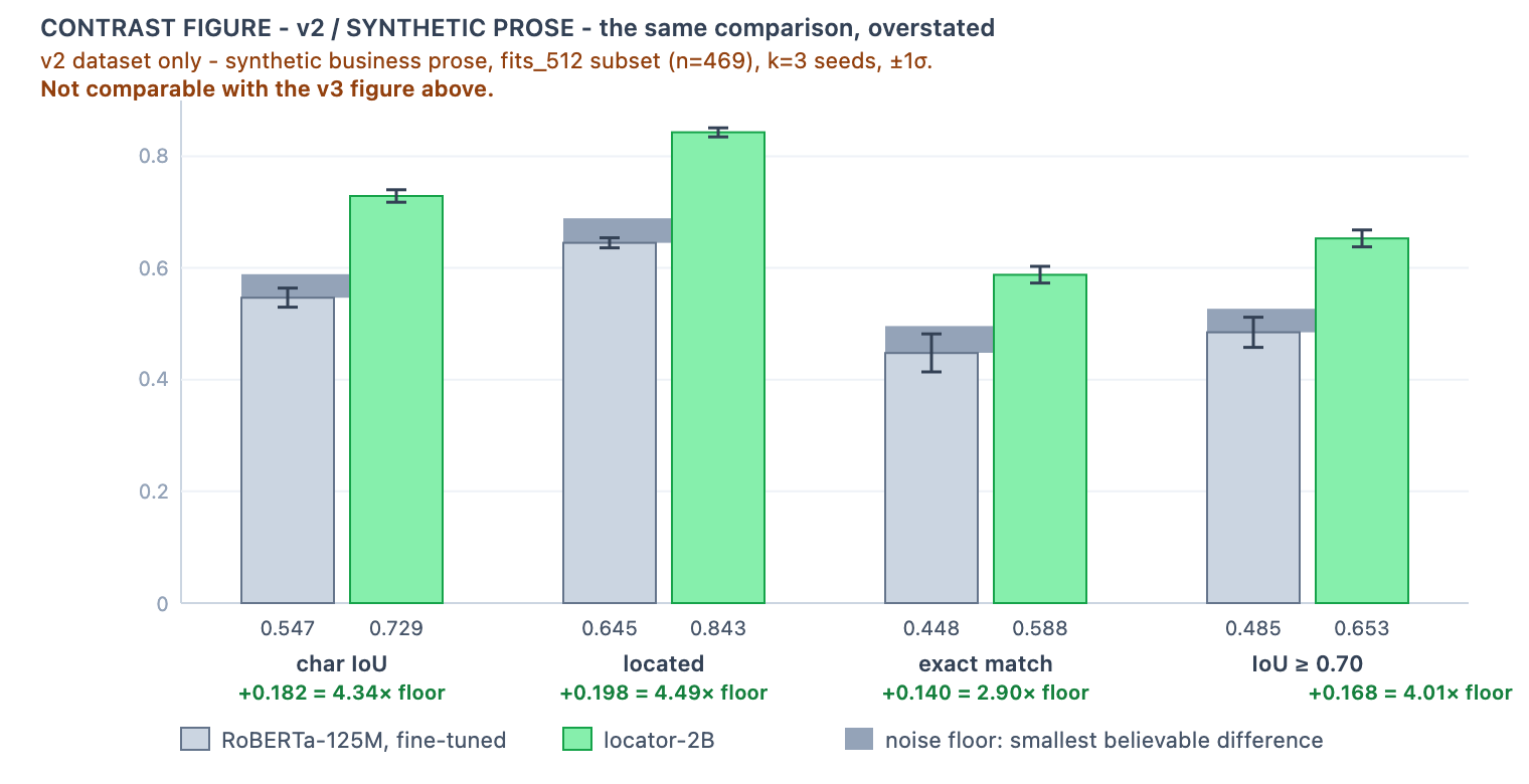The same comparison on synthetic documents. Not commensurable with the figure above, different test set.

My synthetic benchmark was overstating the gap in favour of my own architecture by roughly five times, and I would never have found out if I hadn’t rebuilt the dataset on real prose and re-run the baseline. The old result wasn’t sloppy, three seeds, error bars, 4.3× its own measured noise floor. It was just measuring something other than what I thought. (The two test sets aren’t commensurable, so please don’t subtract one number from the other. Read them as “synthetic” and “real”, not “before” and “after”.)

So what is the real difference? Two things…

Generalisation. On familiar material the encoder is within 0.04. Point it at an entire corpus it has never seen and the gap nearly triples, to +0.098 on the same fits-in-the-window basis. On unseen question categories, +0.091. Same models, same harness; the only variable is distance from training. The defensible claim isn’t “the encoder can’t parse nuance”, it’s “the encoder generalises worse to unfamiliar material”, which is narrower, and more useful, because unfamiliar material is the normal case. You don’t get to pick what your users paste in.

Abstention. This is the bigger one… On held-out question categories, RoBERTa wrongly refuses to answer 15.86% of answerable rows. The locator does it on 3.26%. On the unseen corpus it’s 10.12% against 0.76%. Locating a span you can see is partly a matching problem. Concluding that nothing in three thousand characters of parliamentary debate answers the question requires having understood all of it, and that’s where the extra parameters are actually going.

How do I know my benchmark isn’t lying to me?

Given the above, this is the part I now care about most. The modelling is the easy half.

I run nine gates against every build, five of which are deliberately stupid strategies that shouldn’t work: pick a random sentence, always guess the middle of the document, BM25 keyword match, highest-IDF sentence, reuse the nearest question’s offsets.

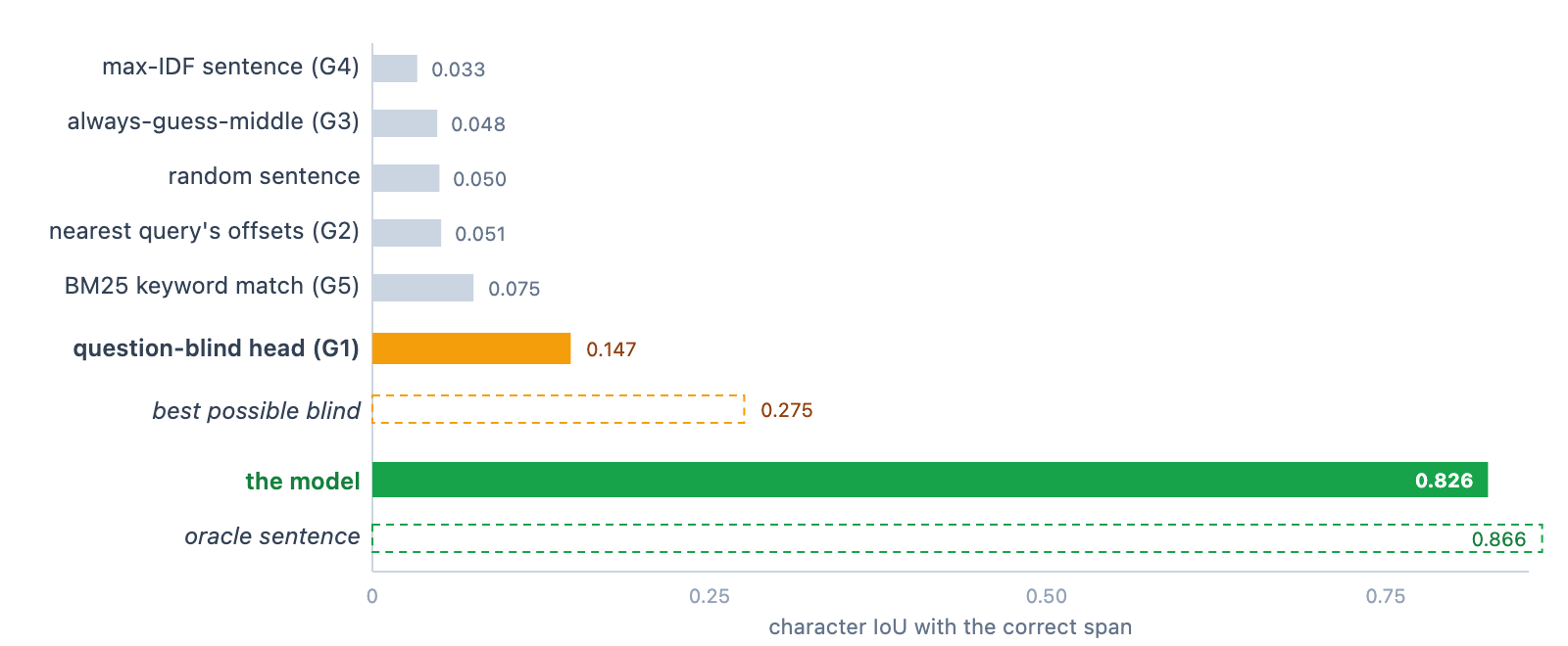Five stupid strategies, a question-blind control, and the ceiling each of them could reach.

They all land between 0.033 and 0.075. “Always guess the middle” mattering was a genuine worry, real prose has strong lead bias, and it didn’t work. Keyword matching gets 0.075 rather than the zero you might naively hope for, and the reason is pure geometry: gold spans here are clause-to-sentence sized, so any sentence-picker earns partial credit just for returning a sentence. Which is why that gate is a lift over a measured floor rather than an absolute. I got that wrong the first time and had to fix it.

The gate I’d actually put in front of a sceptic is the question-blind one. I trained the weak linear head I described earlier, the one whose output is mathematically independent of the question, so it is blind by construction rather than by instruction. It can’t be talked into cheating and can’t accidentally be shown the answer. A blind model’s best possible strategy is to learn one well-chosen span per document, and that is precisely what it does:

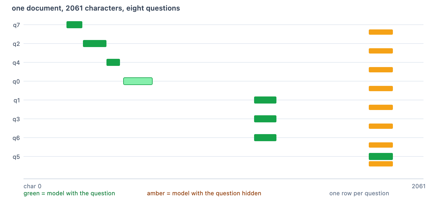Green moves with the question. Amber cannot, so it doesn’t.

One document, eight independently written questions. The green marks move. The amber marks don’t, the blind model returns [1778:1902] for all eight, identically. It happens to be right once, so it scores 1.000 on one row and zero on seven. Across the test set it gets 0.1469 against the real model’s 0.8263.

The stronger version of that argument needs no threshold at all: compute the single best constant span per document, which is the ceiling for any question-blind predictor, and for this split you get 0.2753. The real model sits 3.00× above the best any blind system could ever do.

The honest loose end: the blind model still reaches 53% of its own ceiling, and I don’t know why it’s that high. I’ve tested and rejected two explanations, per-document gold coverage, and gold spans clustering within a document (mean pairwise gold IoU is only 0.072). That one’s unresolved.

For calibration against the previous dataset: the same blind control scored 0.826 there. That’s how I know v1’s benchmark was broken, and it’s the single most useful instrument I built.

Does it know when to shut up?

This is the result I didn’t set out to get and would least like to lose.

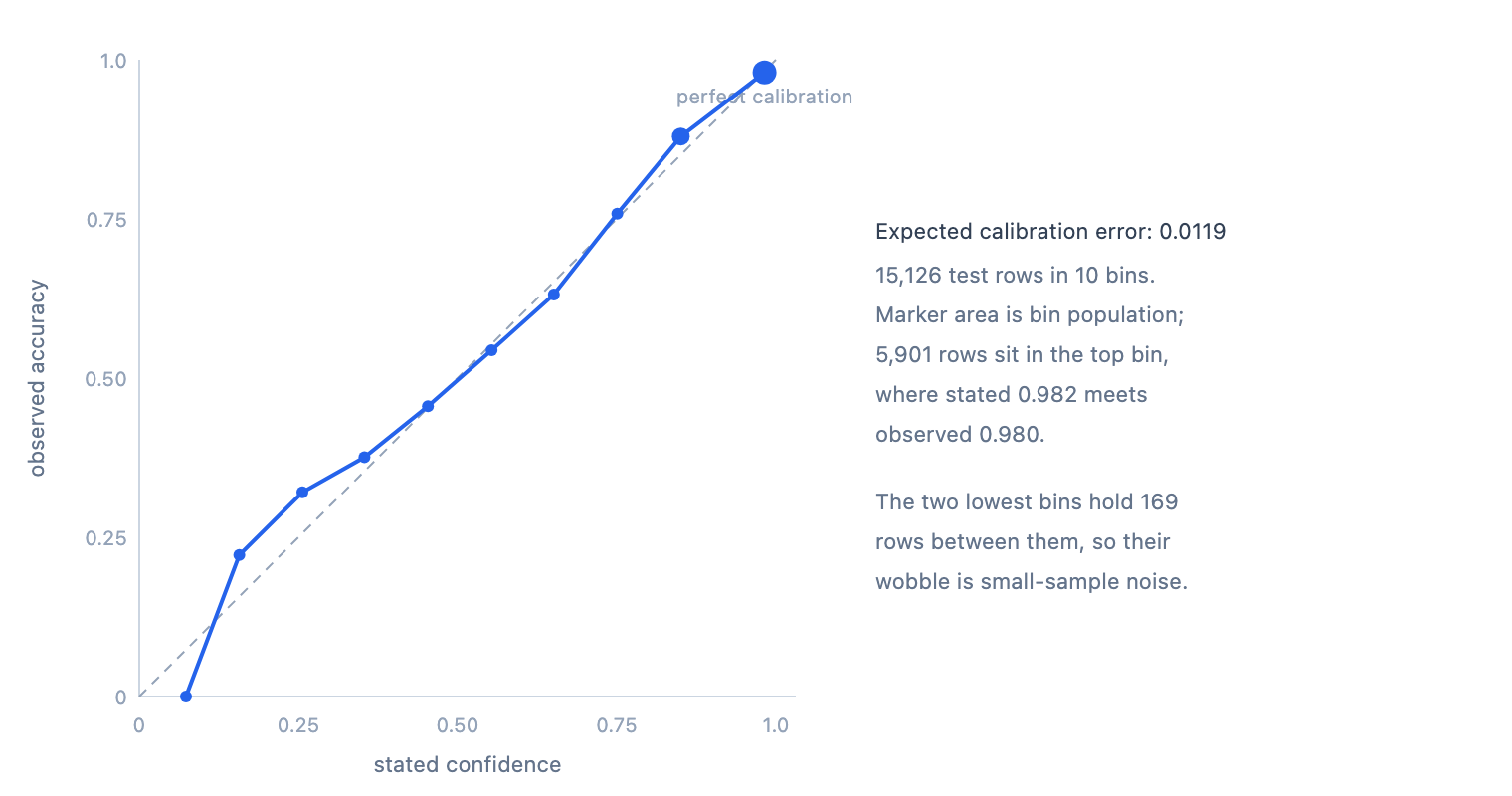Expected calibration error 0.0119. The confidence score means what it says.

Expected calibration error 0.0119 over 15,126 test rows. A confidence score that tracks accuracy to about a percentage point is what lets you put the thing behind a threshold and route the uncertain cases to something slower and cleverer. That’s the property that makes a small model usable as a component rather than a curiosity.

Some of the things I tried

• A SQuAD warm-up curriculum. On the old 2,103-row dataset the model overfit badly and needed this to work at all. At 46,402 rows it’s worth +0.0009 char IoU, nothing. It buys early convergence speed, not final quality. A crutch I can now throw away.
• 0.6B instead of 2B. Costs 0.058 char IoU. Real, outside noise, but it doesn’t settle any argument on its own. The interesting part is that abstention degrades much faster than location: null F1 0.9815 → 0.9540, calibration error 0.0119 → 0.0324.
• A minimum-vocabulary-overlap filter on unanswerable questions, on the theory that more overlap makes a better near-miss. It rejected 62% of them and kept exactly the ones that reintroduced a shortcut. Replaced with distribution matching.
• My best demo. A support transcript where the customer never says they’re leaving, found exactly where the encoder abstains. I had to withdraw it: three of its four questions share one gold span, so a constant-span model scores 0.75 on it by construction, and the blind control does exactly that. A system that provably cannot read the question passed my showcase example.

What’s still weak

Every locator number above is one seed per arm. The RoBERTa baseline is three, which is part of why I trust that column, but mine isn’t. Last round I measured ±0.023 seed-to-seed, which is wide enough that single-seed differences of 0.02 mean nothing, and it bites the 0.6B-versus-2B finding hardest. Four arms ordering as intuition says they should is weaker evidence than three seeds of each, and I haven’t paid for three seeds of a thirteen-hour run yet.

All four corpora are English public-record prose, so cross-domain transfer is untested. And the gold spans were proposed and verified by models, which is circular unless you check against other families. I do that as a build gate: a cross-family panel locates the same passage 0.872 of the time, but agrees on its exact extent only 0.668 of the time. So “where does this clause end” has a real ceiling near 0.67, and the higher extent figure I published on the previous dataset was a Claude-panel number rather than a family-neutral one. That correction runs in the model’s favour, which is exactly why it needed checking by someone other than me.

One more, because it’s a good illustration of why I keep re-deriving my own numbers. An earlier version of the comparison above had a 0.006 discrepancy on one cell that I’d flagged and not chased. It turns out my scoring harness joined rows by id, and 30 rows in the held-out EDGAR split share an id with a different question and a different gold span, so 30 rows were being scored against the wrong answer. My own dataset notes had already written down the warning: any code that keys rows by id will silently drop 67 rows. I wrote that, then walked into it. Fixing it moved the result slightly in my favour, which is the least interesting thing about it.

Lessons

The modelling was the easy part, and I don’t think that’s a statement about this architecture. Every genuinely useful thing I learned came from an instrument built to prove me wrong: a control that can’t read the question, a measured noise floor, a cross-family ceiling, a baseline given every advantage I could think of. The 5× finding is the whole post, and it exists because something in the harness was capable of producing it.

Give yourself falsifiable instruments and you’ll turn them on your own results. Skip them and you get a confident write-up nobody can check, including you.

The other lesson is the one I started with. This took a frozen 2B torso, 19.45M trained parameters and a GPU I rent by the hour. A whole class of language task is sitting there waiting for someone to point a small model at it, and the pattern is already open.

I’d quite like the toolkit to fill up faster.